Grasping the MapReduce Algorithm
6th of September 2016With the introduction of Big Data as an important company asset used in the strategic and tactical decision making, the need has arisen to optimize search and aggregation jobs, or in fact any manipulation for which these large datasets would result in extended computation times. In order to tackle this performance issue, Google introduced the MapReduce algorithm. The idea is to render computation tasks capable of being divided over distributed resources. In order to do this, the computation is redefined in two steps: Map (filtering and sorting the available dataset and partitioning it into a usable subset) and Reduce (aggregating the sorted partitions into a usable result).
The idea for this isn’t brand new. Functional programming patterns, not to mention several algorithms going back to the early days of Dijkstra and Knuth, make use of such an approach. But since 2010, it has really taken hold of current day data calculations and has become the de facto algorithm. Since the Google MapReduce version, many other implementations have popped up and have been integrated into almost all NoSQL databases.
A good way to get some basic insight into the MapReduce algorithm is to watch the episode of the NoSQL tapes on MapReduce with Mike Miller from Cloudant. This episode details both parts of the algorithm, and for those of you that which to read the synopsis instead of the video, I’ll summarize it here.
The Map part of the algorithm consists of parsing all entries in all available datasets and creating a key/value pair for each of these. This is cutting up the large volumes of data into partitions containing the relevant data needed for the computation at hand. Suppose we need to determine the percentage of loan applications that exceeded a certain number (say 500K €), we would map each entry of each dataset into the key/value pair amount/1. This part of the algorithm is extremely suited to have it be done in parallel by different resources in a cluster. These pairs are added to a repository and are usually sorted according to the chosen key.
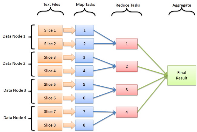
The Reduce part will then take these partitions and execute a calculation (sum of all pairs with a key above 500K €) on this key/value list. In the most basic of setups, this reduce job is executed by a single resource. However, if the partitions are sensibly chosen, even this part of the computation can be performed in parallel by multiple resources. One extreme case presents itself when there would be no Reduce part, and that the key/value pair list is the desired result of the job. This could for example be used to calculate indices to use in databases.
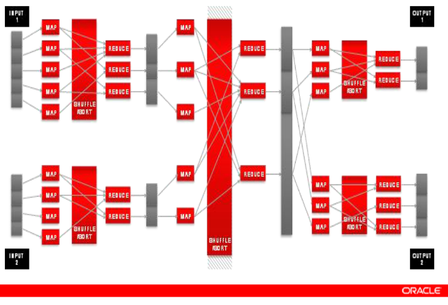
As shown in the illustration below (taken from an Oracle slide deck), these two parts need not be singular in nature. Veritable chains of these MapReduce jobs can be constructed to come up with the proper result for complicated questions, or one might even set up a single Map job to be followed by multiple Reduce jobs taking advantage of the key/value pairs being generated to deliver answers to very different queries.
It is clear that the different implementations of MapReduce shield its users from the difficulties of distributed computing: issues such as resource allocation or dealing with the risk of extensive worker failures and being fault tolerant enough to deal with this. It is a logical addition to the arsenal of the developer needing to perform these types of intensive calculations, a will stay relevant in the land of custom development as well as data analytics for some time to come.
| Thought | EIM |